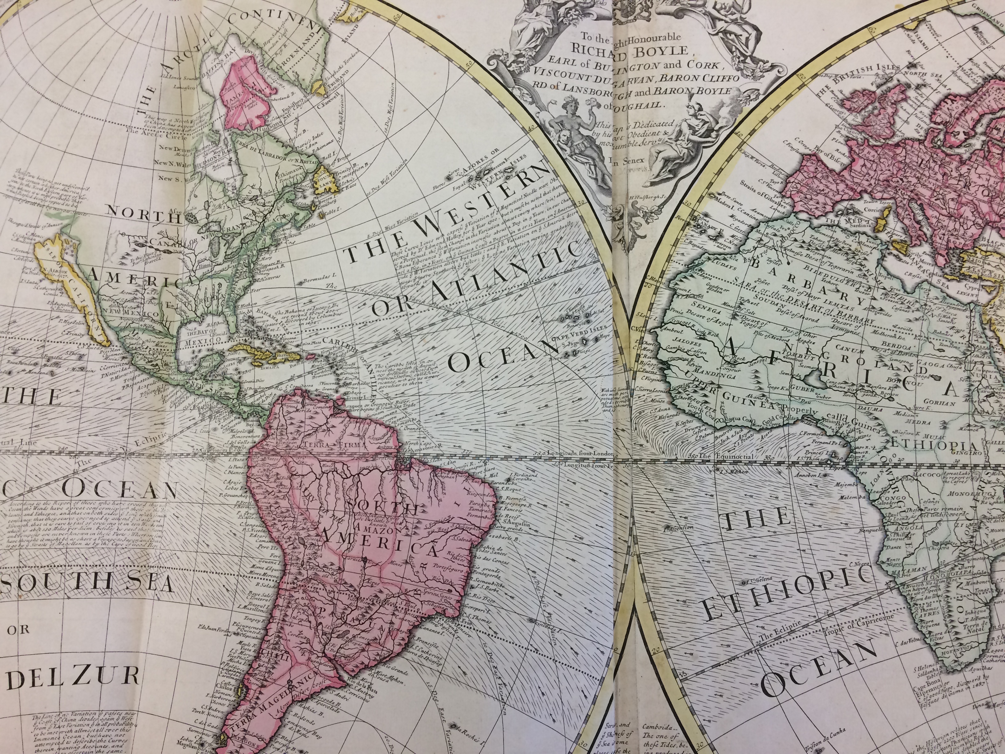
In a time of uncertainty here on Earth it’s reassuring to look to the heavens for a more stable environment, one in which we can predict what will happen with remarkable accuracy considering the vast expanse of space. This amazing map, ‘A scheme of the Solar System with the orbits of the Planets and Comets belonging thereto, describ’d from Dr. Halley’s accurate table of Comets…founded on Sr. Isaac Newton’s wonderful discoveries, by Wm. Whiston, M.A.’ shows with a great amount of information how a complex system of orbits and planetary bodies work together and present a predictable path through time and space.

‘A scheme of the Solar System with the orbits of the Planets and Comets belonging thereto, describ’d from Dr. Halley’s accurate table of Comets…founded on Sr. Isaac Newton’s wonderful discoveries, by Wm. Whiston, M.A., 1712, (E) A1 (3)
William Whiston (1662-1752) was for a time Lucasian Professor of Mathematics at Cambridge University, and he also lectured on Natural Philosophy in London. He produced this map in 1712 with the noted map and globe maker John Senex to illustrate the course of comets as predicted in work by Sir Edmund Halley and the ground-breaking work on planetary motion set out by Sir Isaac Newton.
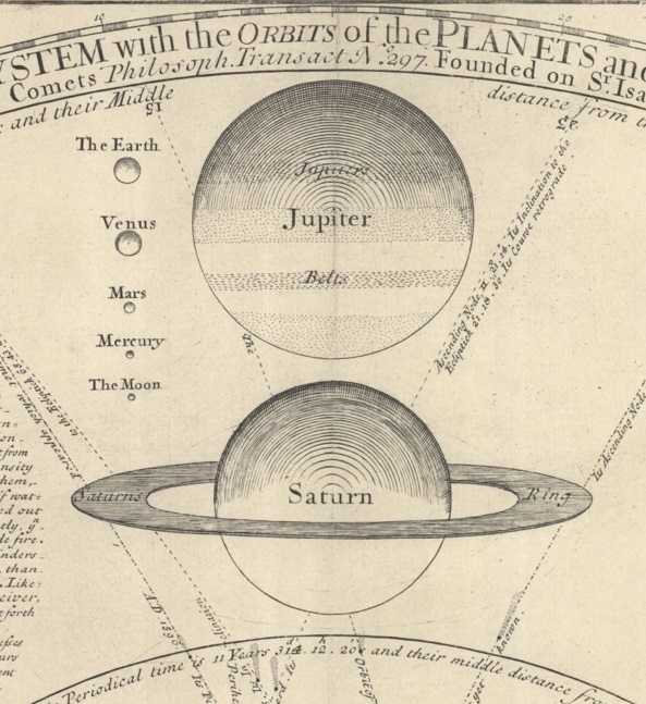
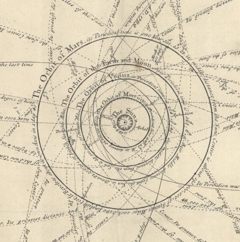
The map shows the orbits of ‘about twenty one known Comets…’. according to Halley’s calculations (there are now over 3,000 recorded Comets in the Universe), the orbits of the Planets and, at the top, the relative size of the 6 known primary Planets and the Moon (the size of the Sun is represented by the outer circle of the map of the Solar System).
There is a remarkable amount of explanatory test on the map describing the six Planets and the ten secondary Planets (which we would know call the moons of the Earth, Jupiter and Saturn) and descriptions of the system of Comets and the Sun. Like all good exponents of a new theory Whiston makes a bold claim for his map at the start. ‘I do here, good reader, present thee with a scheme of the Planetary and Cometary World, part of which hath of late been called the Hypothesis of Pythagoras or Copernicus, but is now so certainly known to be the real system of nature that it ought no longer to have that uncertain title of hypothesis applied to it’. It’s amazing how many maps produced around the 1700 and 1800s include some form of claim such as this, or include in the tile ‘A new survey..’ or a variation on that phrase. The text goes on to acknowledge the size of the Universe and then ends with crediting the Creator, ‘As to the Fixed Stars, they are vastly remote from our Planetary and Cometary system but may perhaps every one be the center of another Solar System. Dr. Hook and Mr. Flamsteed think they have discovered their annual parallax and that is about 45″ which will imply there to be 900,000 millions of miles distance from our Sun; or according to Hugenius’s calculation in the like case much further than a bullet shot out of a canon could go in 100,000 years. But of such vast and numberless systems…we know very little, only so much we know of ye Planetary and Cometary World, and of the probability of Fixed Stars…as is sufficient to make us cry out with the Psalmist O Lord, how manyfold are thy works! In wisdom have you made them all!
Robert Hooke (1635-1703) produced most of the surveys of London after the Great Fire of 1666 and went on to try and measure distances to stars using parallax, which takes the difference in angles of a measured distance seen from two different points. John Flamsteed (1646-1719) was the first Astronomer Royal and wrote star atlases and catalogues which were more detailed than any previously published. Hugenius is the Latin version of the name of the Dutch polymath Christiaan Huygens (1629-1695), one of the leading scientists of his or any other age. One of Huygens many contributions to science was the discovery of Saturn’s ring system and the first of the Planet’s moons after making improvements to the telescope. Hooke and Halley were involved in a wager offered by no less than Sir Christopher Wren while the three were at lunch in 1683 to discover why the Planets orbited the Sun in an ellipse, and not in a circle as suggested by Copernicus. To find the answer Halley travelled to Cambridge to talk to Isaac Newton, at the time Lucasian Professor of Mathematics ( Whiston replaced Newton in the role in 1702). Not only did Newton have the answer to the question but following promoting by Halley wrote his findings up in one of the most important Scientific books ever written, the Mathematical Principles of Natural Philosophy, more commonly known by the first word of the original Latin title, the Principa. In this book Newton set out his three laws of motion and explains how the orbits of the celestial bodies work and the nature of gravity. Newton’s ideas in the Principa and Halley’s work on comets are the key to Whiston’s map.
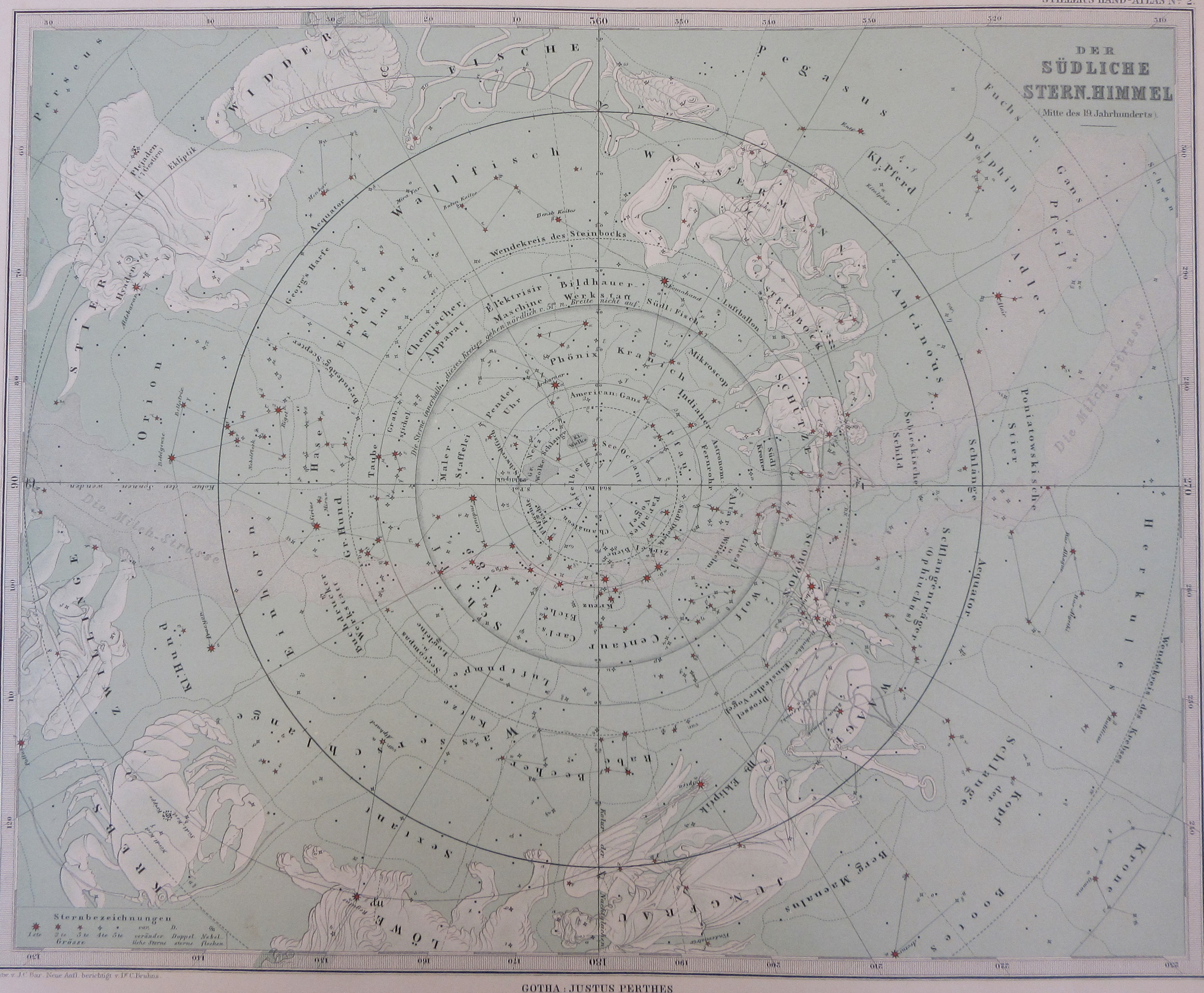
John Senex was a noted map and globe maker and uses text at the bottom of the map to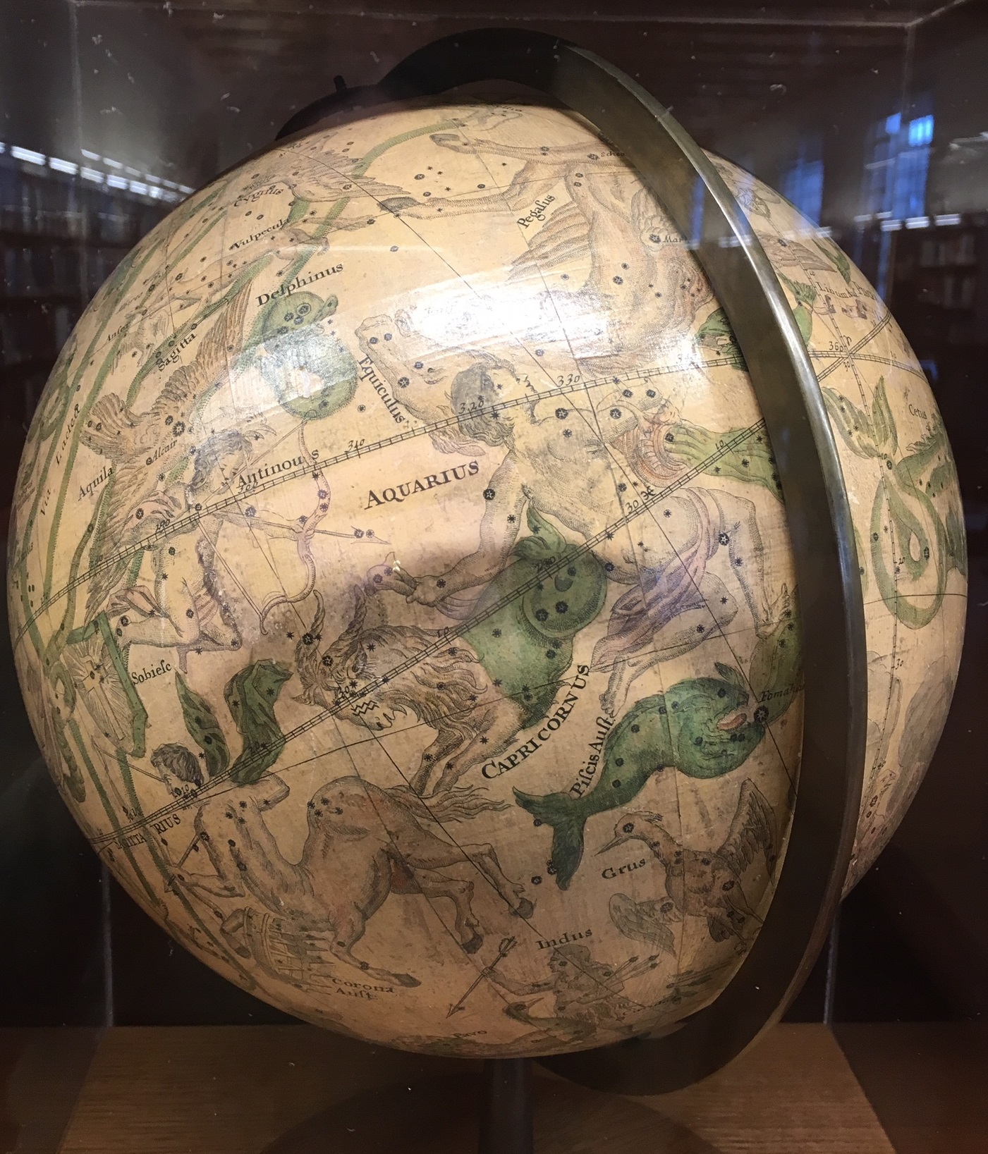 promote his products, extolling the worth of his maps and globes while also warning of the inferior products made by others based on his work. There are two of Senex’s globes on display in the Rare Books and Special Collections Reading Room at the Weston Library (the globe of the heavens is shown here), possibly the two mentioned in the text ‘ He maketh ye newest globes of 16. 12. & 3 inches diam. and has just finish’d in a most elegant manner a pair of 28 inches diam. fit to adorn public librarys, or of the librarys of the most curious’. Senex has featured on this blog before, first in a
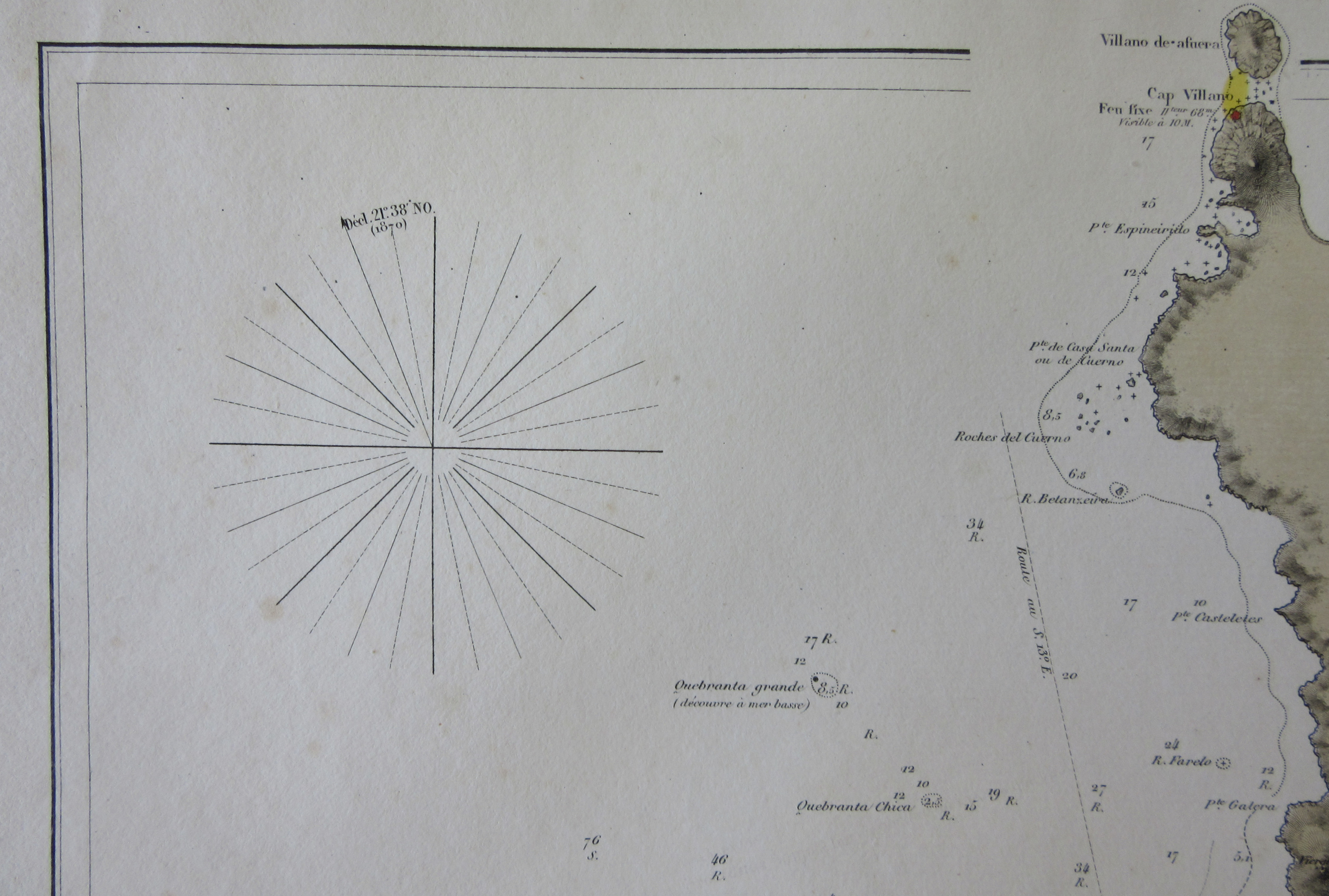
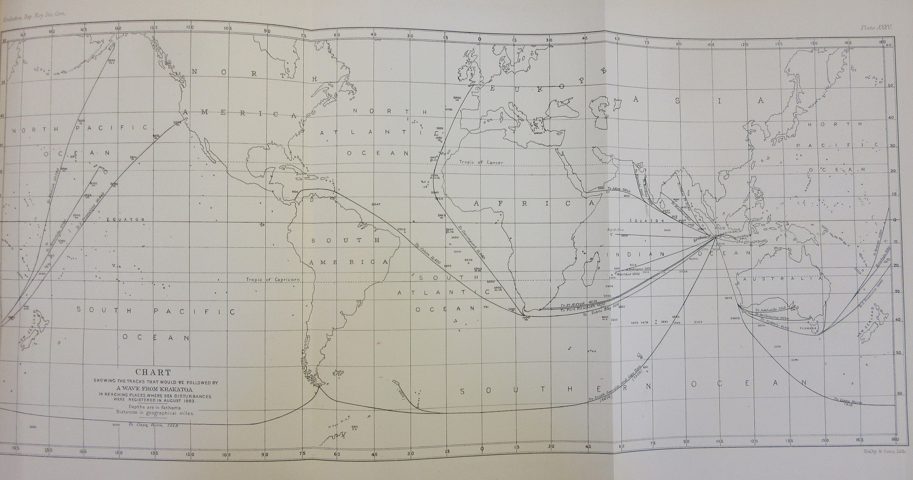
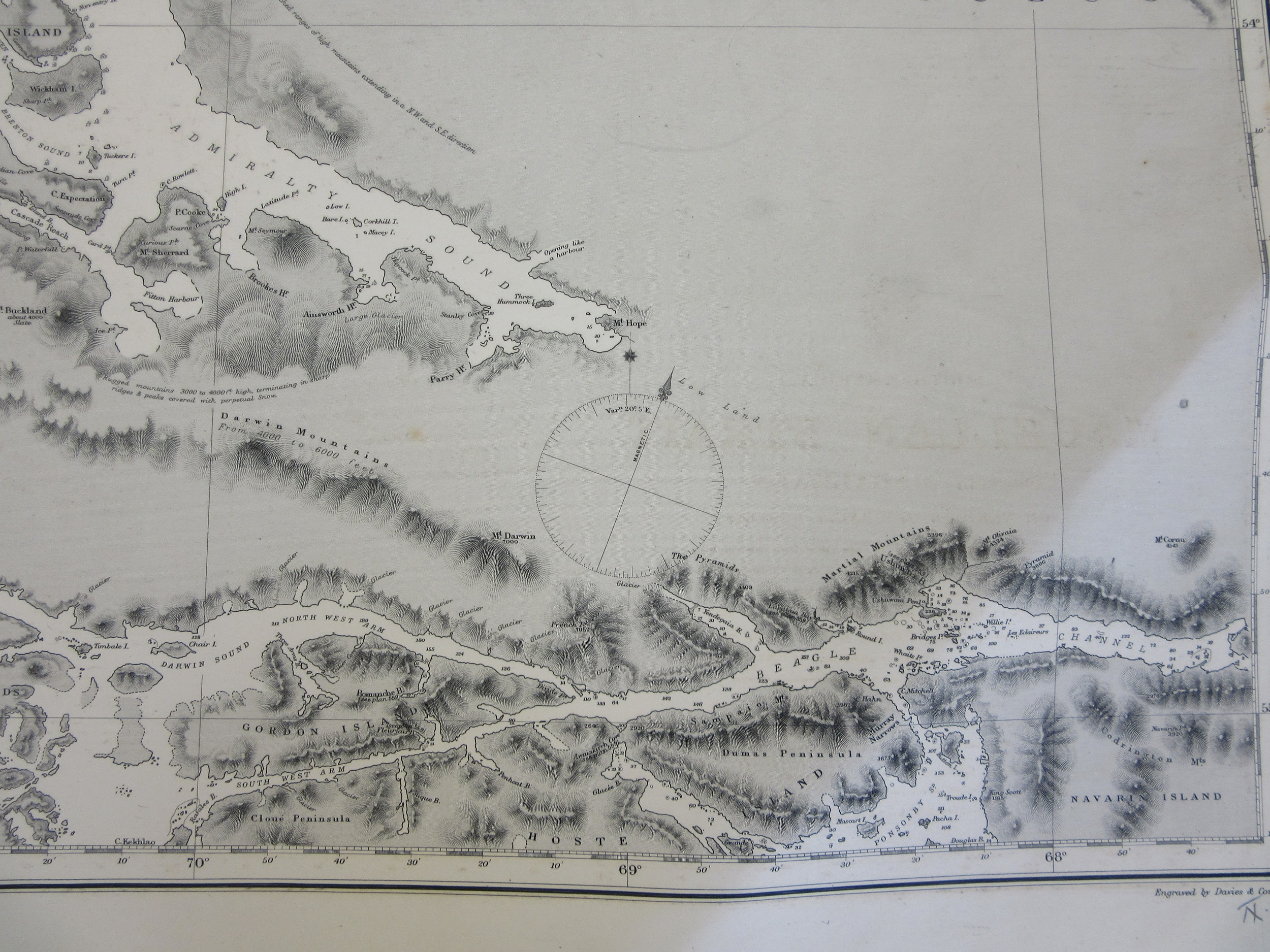
piece about globes (http://blogs.bodleian.ox.ac.uk/maps/2019/01/28/golden-globes/) and then, and more relevant to this piece in a post about a map of South America (http://blogs.bodleian.ox.ac.uk/maps/2019/02/22/a-tale-of-two-maps/) which is dedicated to Halley and marks the point where, during a voyage to map the magnetic variations in the Earth, Halley’s ship the Paramore encountered ice for the first time. Halley then produced a map of the World with the variations shown, which would enable navigators to plot a correct course using a ship’s compass with corrections made according to the variation shown

Halley’s magnetic chart [a facsimile from 1870 of Halley’s ‘New and correct chart shewing the variations of the compass, 1701] (E) B1 (382)


 In Erde und Sonne different diagrams explain the journey of the Earth around the Sun, showing the tilting of the Earth on its axis that gives us the changing seasons. For the purposes of the blog figure 5 is the most important, Lauf der Erde um die Sonne (Erdrevolution), which shows the Earth’s rotation around the Sun. At the top is the Earth in relation to the Sun on the 21st of March, showing a perfect split between light and shade running from Pole to Pole,
 Mary is an important figure in the history of navigation. She is the Pole Star, a constant in the night sky and is also the saint of Navigators and, most useful on a journey, the ‘Virgin of Good Winds’. This image of the Virgin and Child comes from an early Portuguese portolan chart of the Atlantic. The cartouche with Mary in the centre is located in North America, a guide to those making the perilous journey across the ocean to the New World. Circling Mary are the words to the prayer ‘Ave Maria’, a prayer no doubt uttered on many a dangerous moment on-board ships, ‘…pray for us sinners now and at the hour of our death. Amen’.

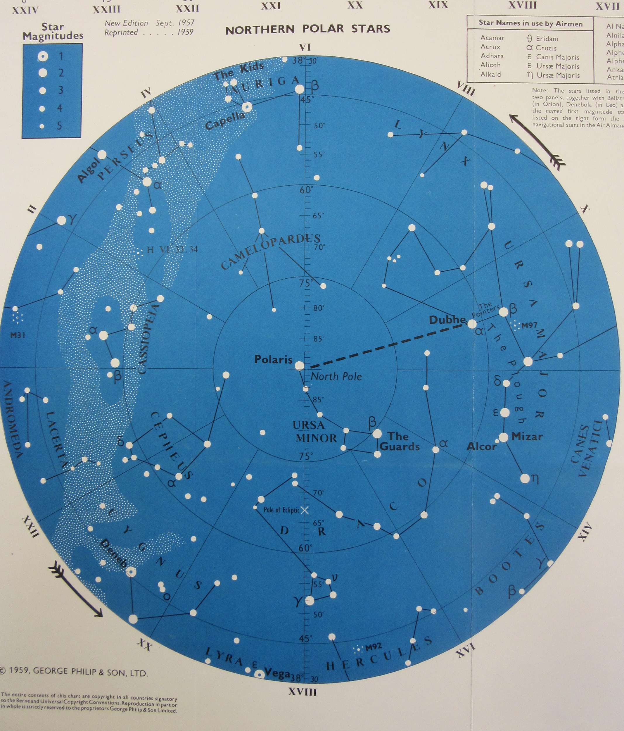


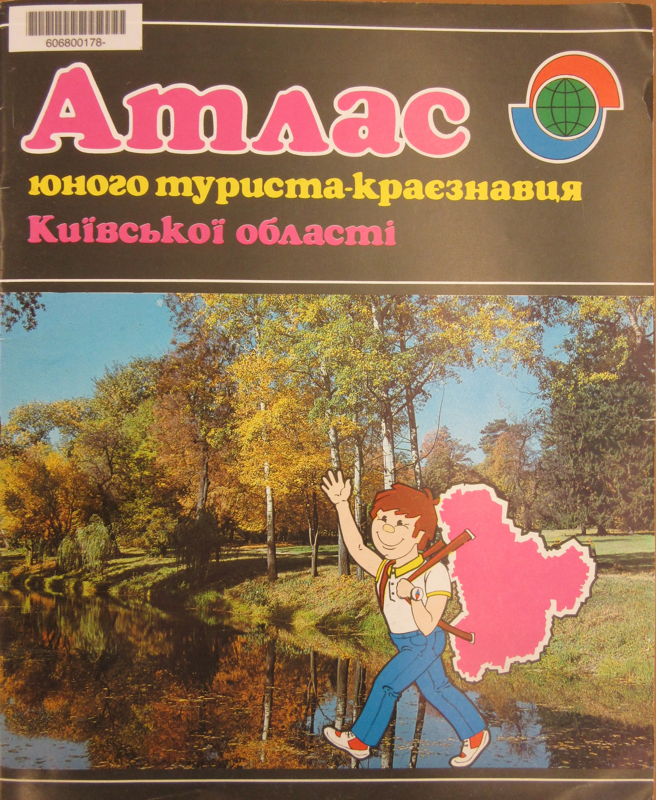
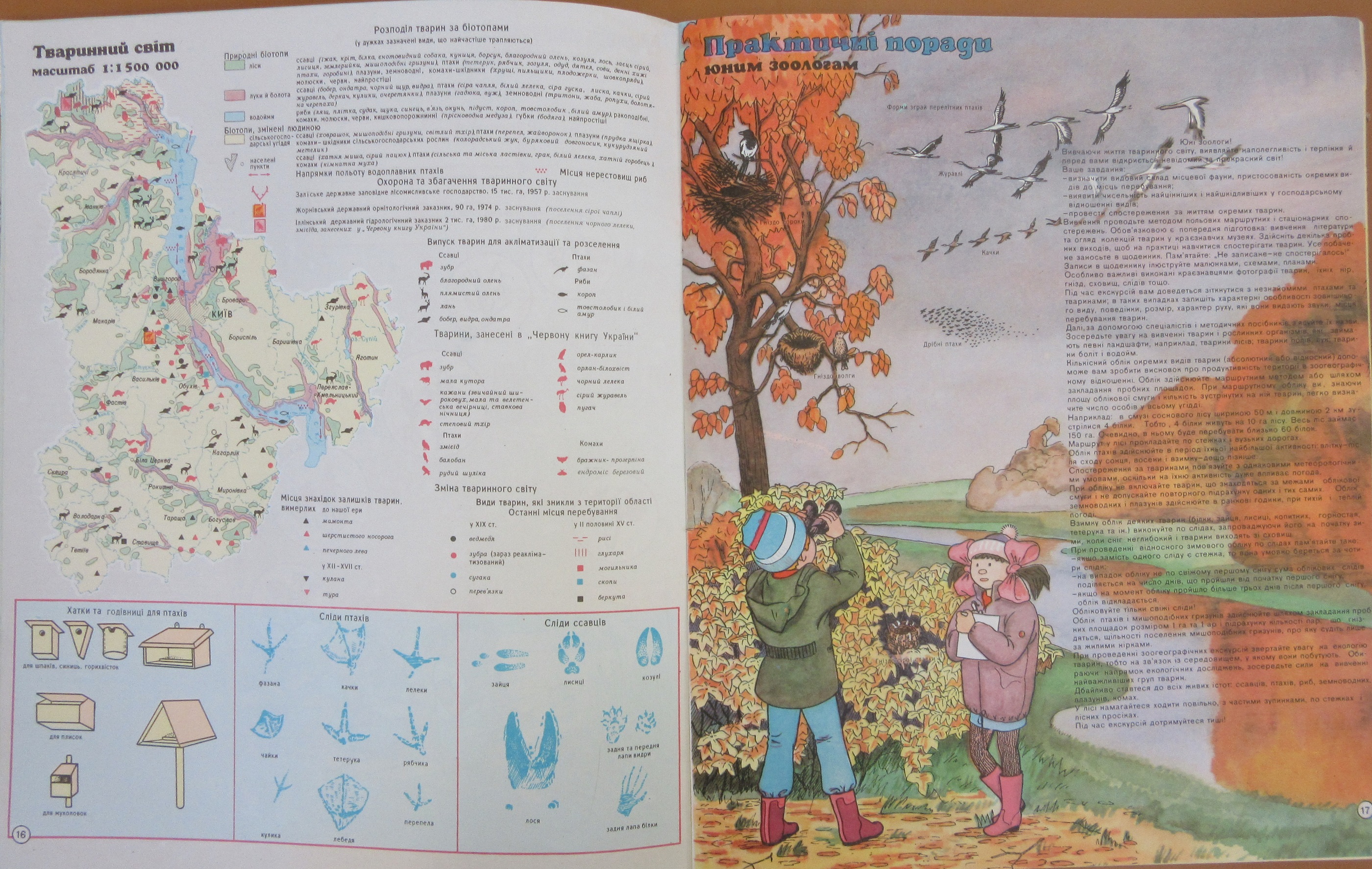

 The atlas also includes illustrations and text on surveying techniques and, shown here, orienteering. Text above the star chart in the top corner shows how you can find north by looking for the Big and Little Dipper in the sky, while notes on the ground explain how studying the landscape can help find direction (мох укривае піеічний біх дерее і каміння, or ‘moss covers the north sides of trees’, for example).